(RADAR)
(RF-HEAD)
(ANTENNAS)
(PROCESSING)
(WEATHER)
(HOME)
Homemade FM weather radar at 10GHz
Matjaz Vidmar, S53MV
4. Signal processing
Signal processing basically includes spectrum analysis of the low-frequency beat signal. In order to achieve the best possible signal-to-noise ratio, a parallel (FFT) spectrum analyzer is recommended.
The described FMCW radar is designed to maintain the low-frequency beat signal within the bandwidth of a typical computer sound card. Using lower beat frequencies would make the system excessively sensitive to the Doppler shift caused by cloud movement. Using higher beat frequencies would degrade the signal-to-noise ratio as well as require much more expensive hardware than a conventional sound card.
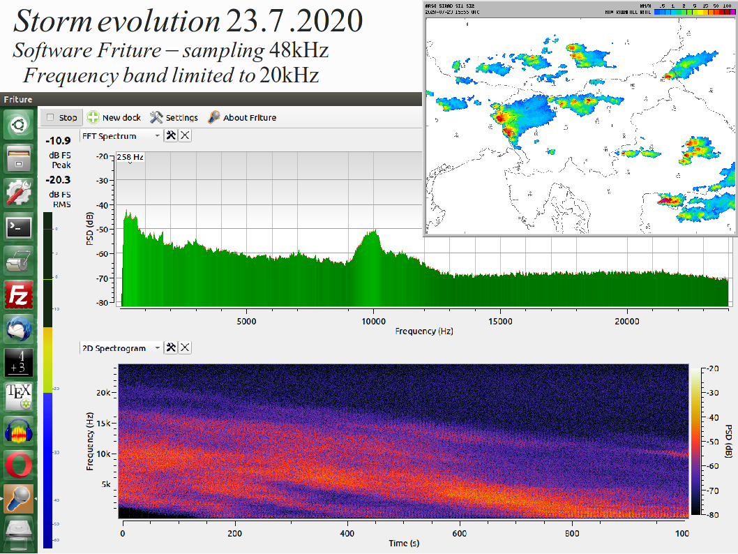
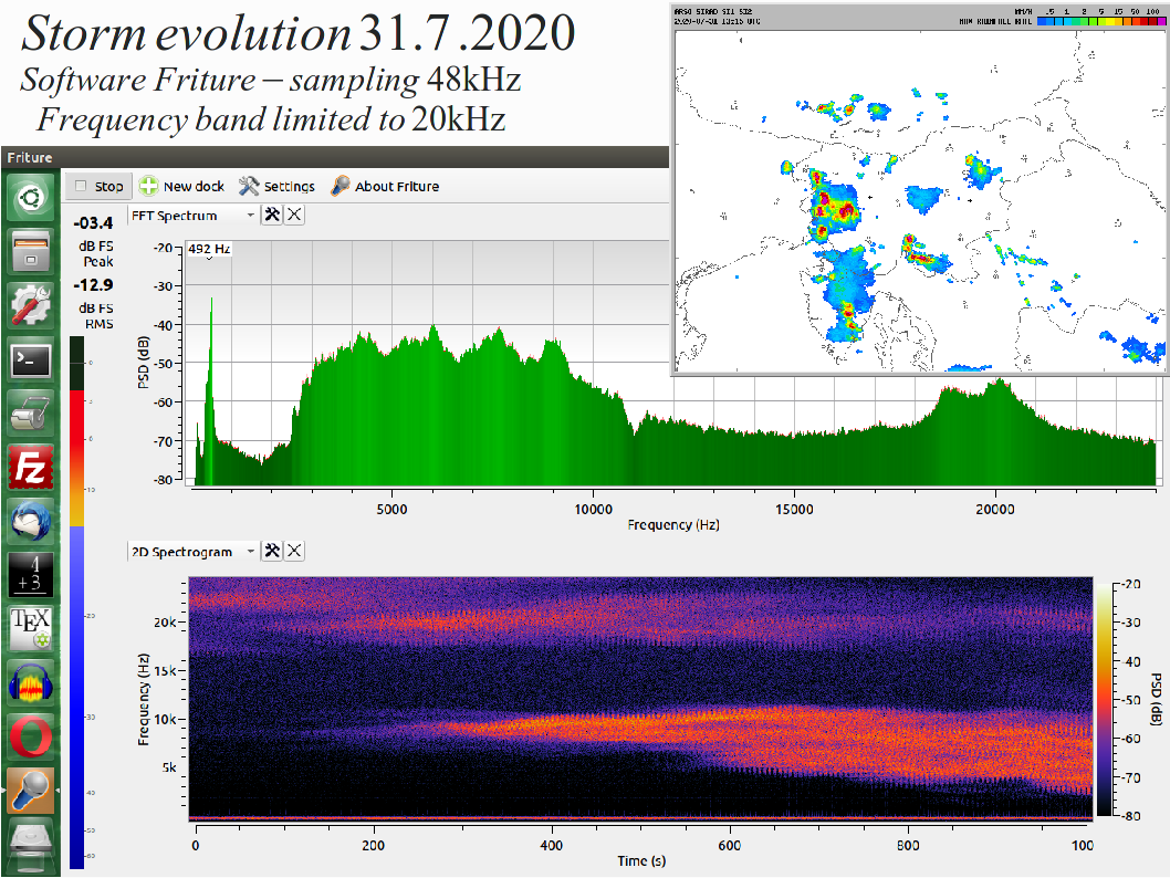
The free software "Friture" allows signal sampling at 48kHz. Further "Friture" allows drawing a "waterfall" spectrogram for the duration of up to 1000 seconds (~17 minutes). Within these 17 minutes the evolution of an approaching thunderstorm can easily be observed:
The corresponding image from a commercial pulsed weather radar is shown in the upper left corner for comparison. A similar storm evolution is also shown one week later. Of course the described FMCW radar only observes the evolution of events in a single antenna direction at both azimuth and elevation fixed, selected manually on the rotor controller.
The described FMCW radar uses both directions of the triangular frequency sweep. The FFT is not synchronized to the frequency sweep. The FMCW frequency shift changes sign on each slope while the Doppler shift does not change its sign. The FMCW sweep frequency is selected so that the Doppler shift of moving clouds remains an order of magnitude smaller. The Doppler shift of a quickly-moving cloud therefore appears as a short-period interference pattern on the "waterfall" spectrogram:
Custom software for FMCW radar signal processing was written in "Python" using extensive math array routines from "numpy" and graphics from "matplotlib". Although "Python" runs on several different operating systems, it is usually advantageous to use some version of "Linux", since the latter allows more programming freedom for soundcards than "Windows".
The interpreter nature of "Python" is not a disadvantage here since any complex programming is available as pre-compiled routines of "numpy" and "matplotlib":

Although a single-channel MIC input is used on the sound card, the "Python" routine "sounddevice" produces a two-channel recording of the specified number of samples. Some older soundcards may not allow a sampling frequency higher than 48kHz. On the other hand, some new soundcards, while allowing up to 192kHz sampling, may require setting the variable "sd.default.device=0" to a value different from zero. A single 47kohm series resistor was found to be the best interface to MIC inputs of many different sound cards. The 47kohm resistor is best installed close to the sound card to avoid picking unwanted noise.
The antenna-rotor interface is accessed through a RS-232 USB dongle located at "/dev/ttyUSB0". Any software is expected to crash if the RS-232 USB dongle is not available!
A raised-cosine window is used in front of the "numpy" "rfft" routine. In order to avoid loosing any information in the signal, subsequent raised-cosine windows are overlapped. Finally the output of "rfft" is squared and averaged to obtain the power spectrum. The averaged power spectrum is further converted a logarithmic [dB] scale:

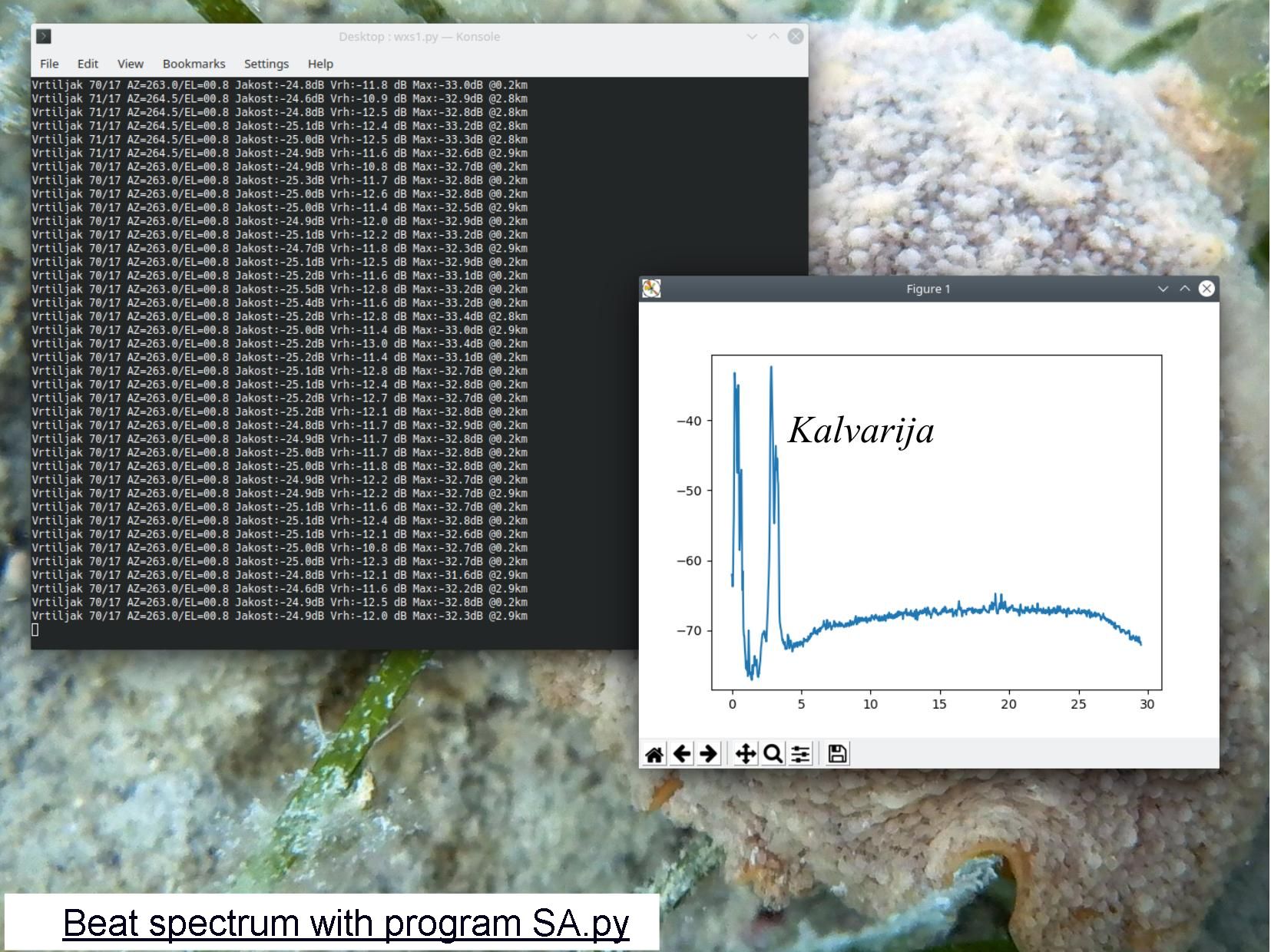
SA.py is a simple audio FFT spectrum analyzer including averaging. If executed without a terminal (console) window, only the spectrum window is shown. The spectrum window is periodically refreshed by "matplotlib" as new data arrives to the soundcard. The FMCW distance beat is converted to [km] automatically. A mouse click on the spectrum will store, report and normalize the image. Any keyboard click in the spectrum window will exit the program.
If the SA.py is executed in a terminal (console) window, additional data is show in this window. This data includes rotor position both as raw counts and calculated azimuth/elevation, the sound card average signal amplitude, peak signal amplitude, spectrum peak and distance. 0dB means A/D converter saturation. No commands are sent to the rotor interface except for reading its status (20 bytes) with the command "P"=80. The terminal window is updated as each new spectrum-data set arrives:
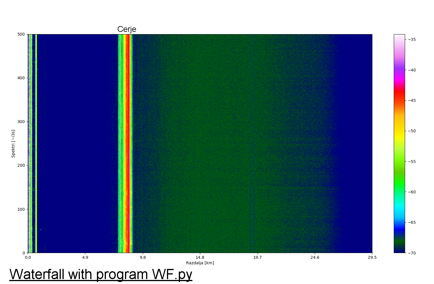
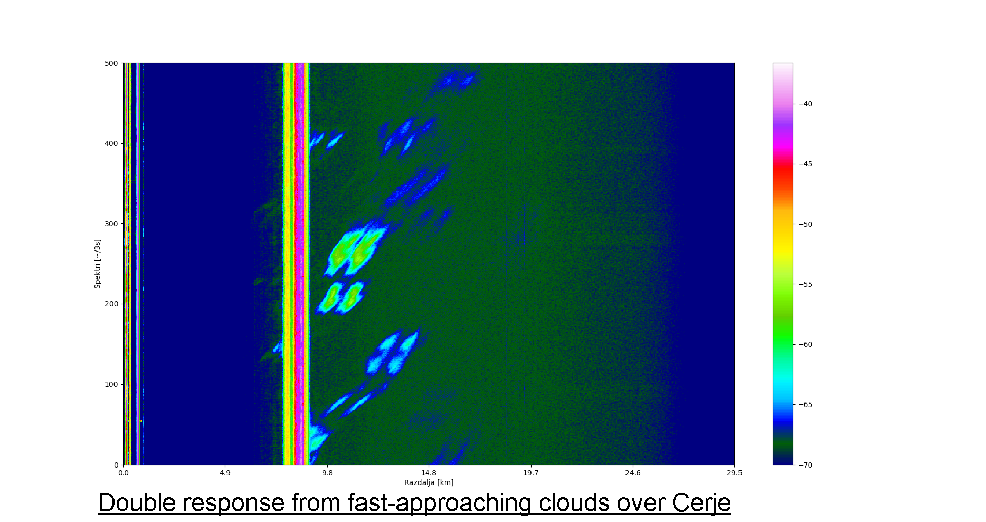
WF.py displays a "waterfall" audio FFT spectrogram including averaging much better than "Friture". If executed without a terminal (console) window, only the waterfall window is shown. The waterfall window is periodically refreshed by "matplotlib" as new data arrives to the soundcard about one line every three seconds. The whole waterfall includes 500 lines of data for the last half hour. The FMCW distance beat is converted to [km] automatically. The colormap "gist_ncar" is used for the amplitude. A mouse click on the spectrum will store the image. Any keyboard click in the spectrum window will exit the program. A fixed reflection at 0.8 degrees elevation from Cerje at 8.7km is visible on the following waterfall:
If the WF.py is executed in a terminal (console) window, additional data is show in this window. This data includes rotor position both as raw counts and calculated azimuth/elevation, the sound card average signal amplitude, peak signal amplitude, spectrum peak and distance. 0dB means A/D converter saturation. No commands are sent to the rotor interface except for reading its status (20 bytes) with the command "P"=80. Image storage is also reported in the terminal window. The terminal window is updated as each new spectrum-data set arrives.
If the target has a significant radial speed of several tens of m/s, two separate responses can be seen from both the raising and trailing slopes of the frequency sweep. Of course no Doppler shift can be observed on the tagential speed of the target. The example below shows the described effect with WF.py on fast and high clouds approaching from south (Cerje) on Nov 16th, 2025:
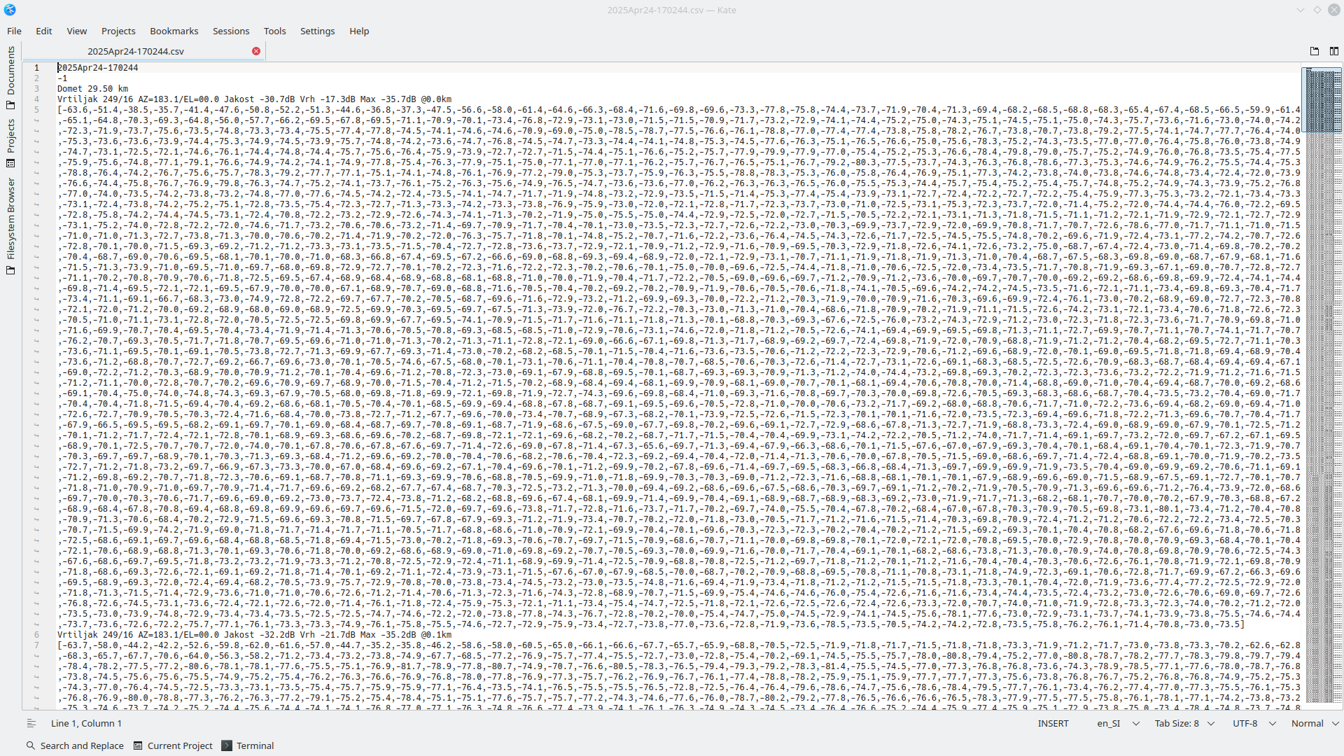
PPI.py generates a plan-position indicator (PPI) graph most familiar to many different types of radar. The main program always runs in a terminal (console) window. The program asks for a file name first. If no file name is provided, the program will start moving the antenna and record a new file first. The name of the new file is derived form the current date and time from the computer real-time clock. The recorded data is plain ASCII text in .CSV (comma-separated values) format:
The measurement should start at one extreme azimuth position set manually by the KR5600 rotor controller. The program then instructs the interface to run the rotor to the other azimut extreme with the command "Q"=51. The antenna rotor runs at full speed and requires approximately 65 seconds for approximately 280 recordings at incremented (or decremented) azimuths. The rotation is stopped while reaching the other azimuth extreme and/or when KR5600 azimuth end-of-travel switches are activated. For sequential measurements PPI.py flips the azimuth direction automatically so that no manual return of the antenna is required.
When the extreme azimuth is reached, the data recording will stop. When a full data set is available, either after recording of a new file ends or while manually inserting an existing file name, the PPI.py program will ask for the radius of the PPI graph to be drawn. The "mathplotlib contourf" function is used for a polar graph together with the color map "gist_ncar". The "contourf" function provides excellent interpolation between adjacent values. A mouse click on the PPI image will store the image and report the storage in the terminal window. Any keyboard click in the PPI window will close it and return to the terminal window asking for a new range.
The maximum range of 29.5km is used if none is provided. From my location clouds could only be seen up to 25km distance due to Earth's curvature. It usually makes sense to use a graph radius of 10km or less. A zero or negative radius will exit the program in a controlled way:
The program WF.py therefore allows observing the evolution of a thunderstorm in a single direction while the program PPI.py provides a much slower PPI display due to the slow antenna rotation. The programs SA.py or WF.py also helps various system adjustments like the antenna elevation, the trimmers in the KR5600 control unit or the sensitivity of the MIC input of the soundcard.
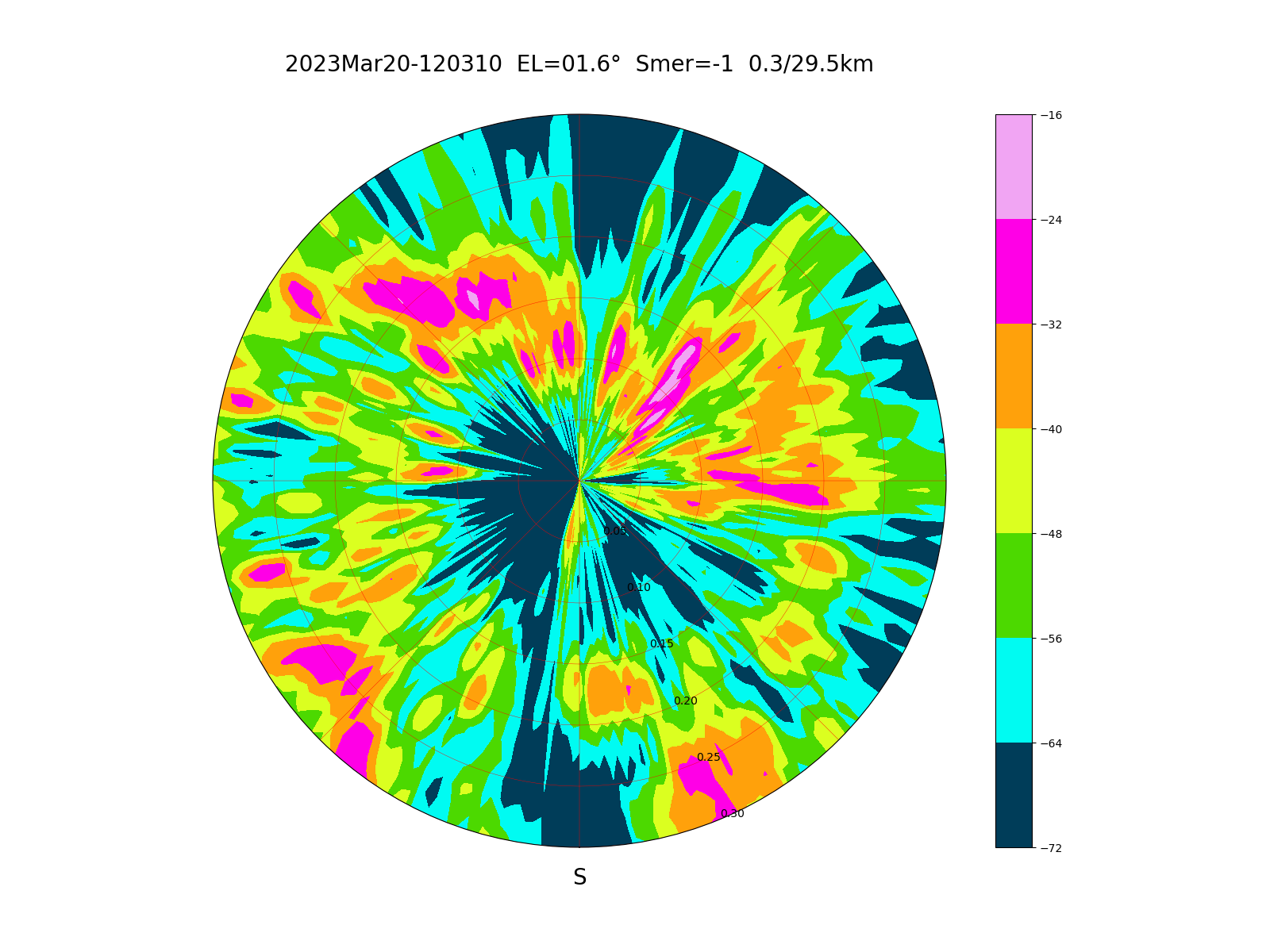
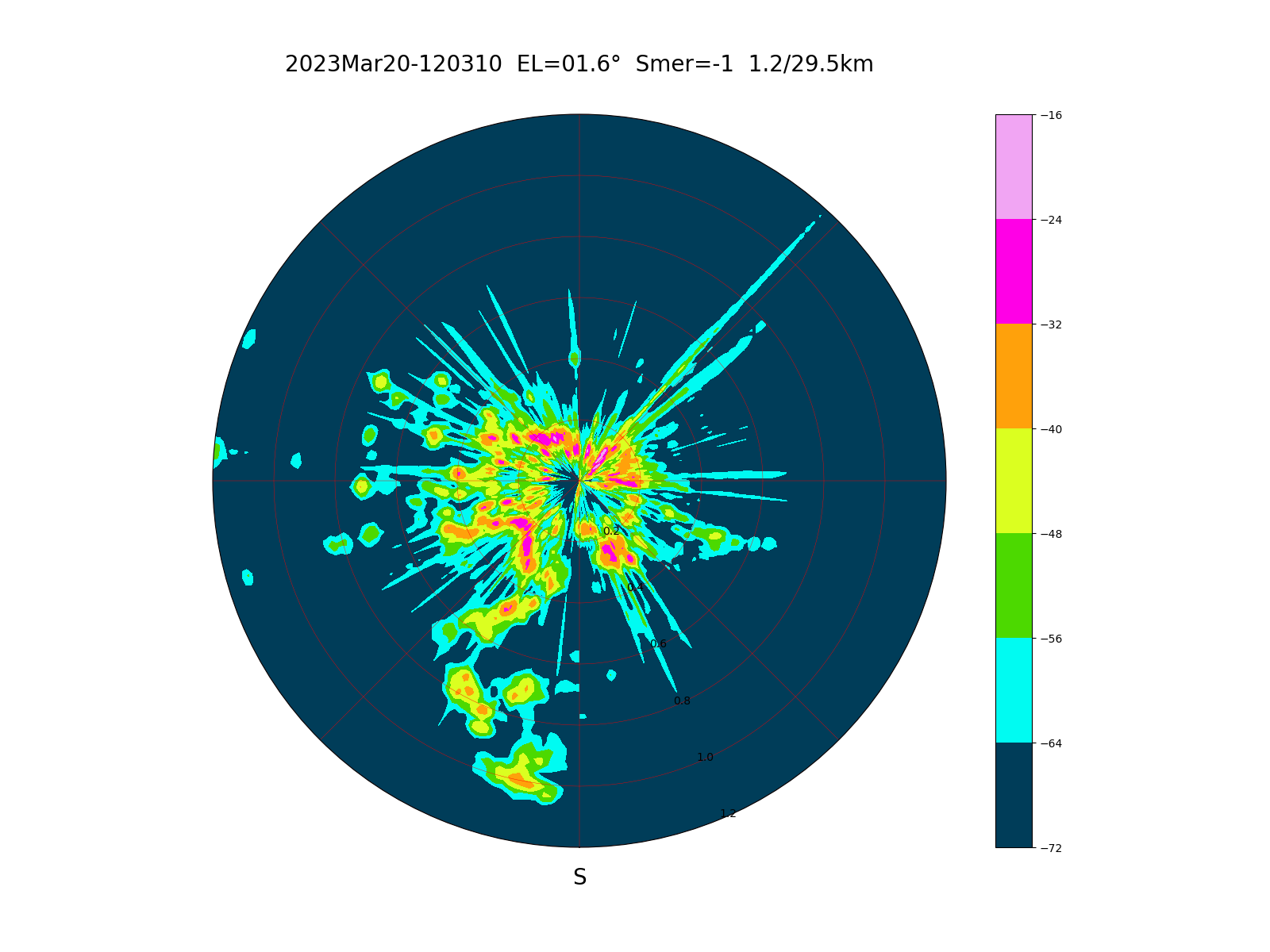
The same recording form PPI.py allows much different PPI images to be produced at different ranges. The following PPI images at low elevation are from horizon obstacles only since no precipitations were present. Within a 300m radius only nearby houses are visible at low elevation:
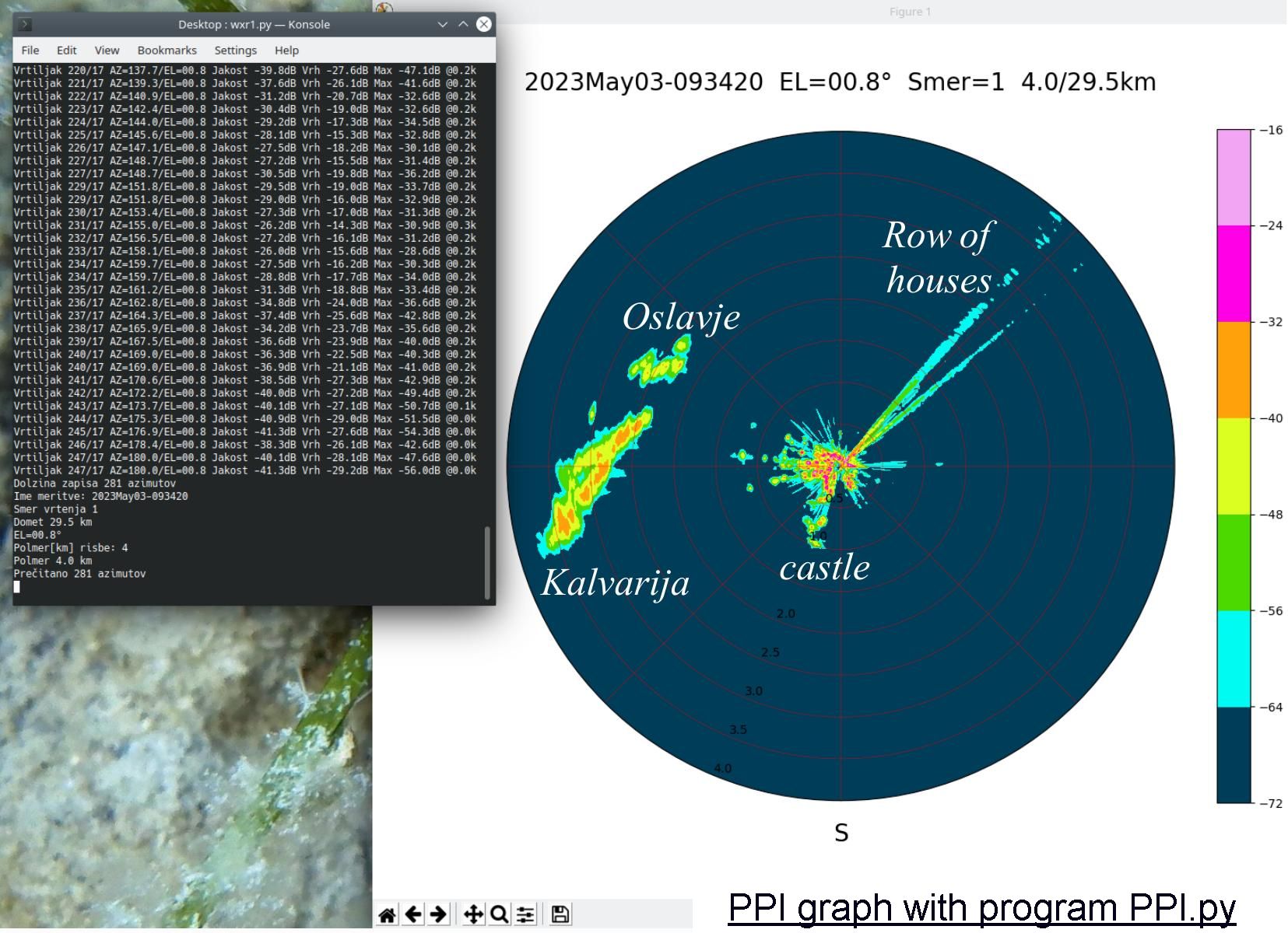
Within an 1.2km radius all houses including the castle to the south are visible at low elevation. Beat harmonics from very strong reflections from rows of houses to the northeast are also visible:
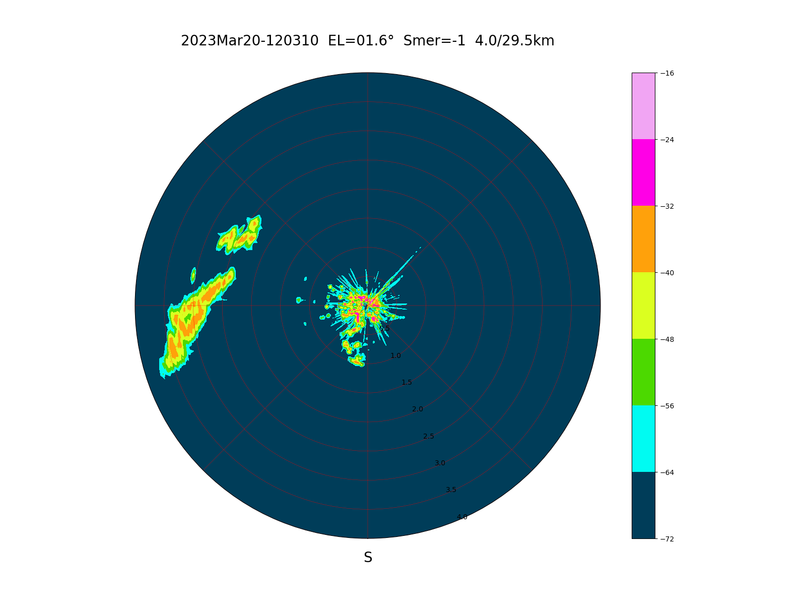
Within a 4km radius nearby hills (Kalvarija to the west) are visible at low elevation:
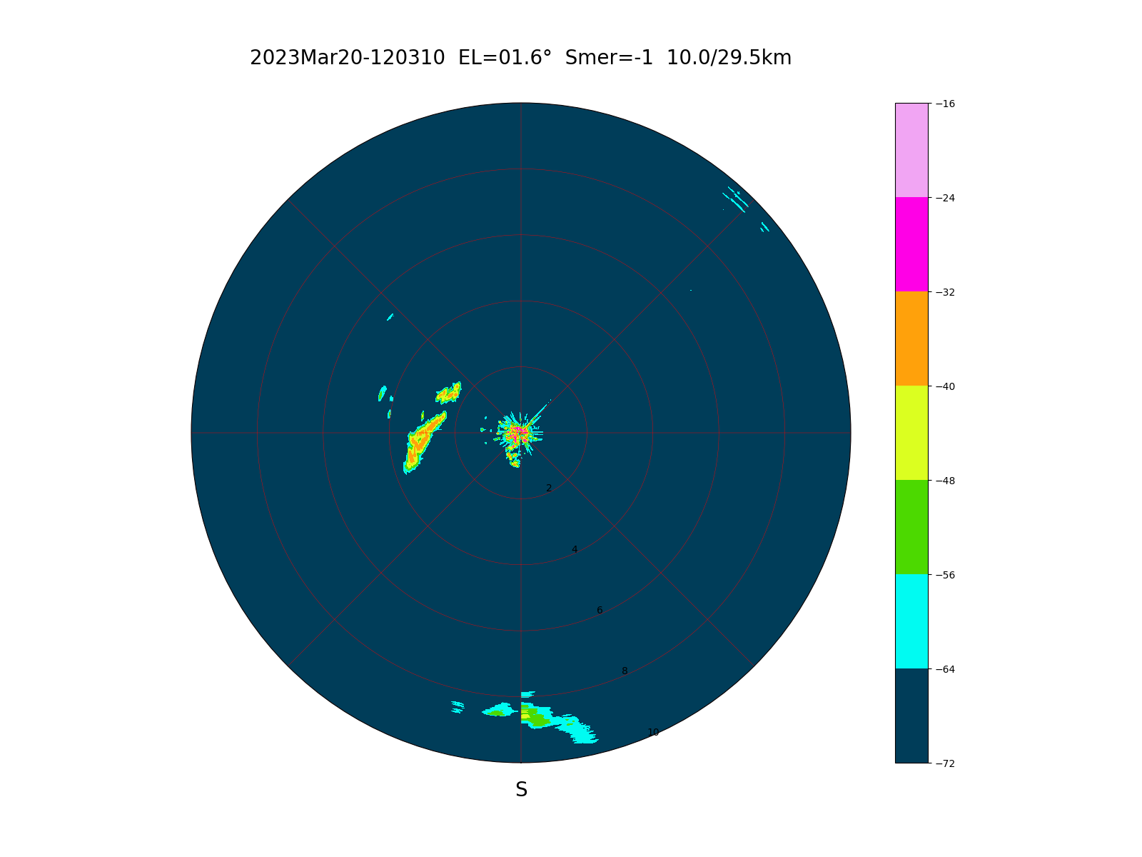
Within a 10km radius hills (Cerje to the south, Steverjan to the northwest) are visible at low elevation. Since the azimuth scan goes from south to south, an imperfect overlap in the south direction is visible when the azimuth rotation angle slightly differs from 360 degrees:
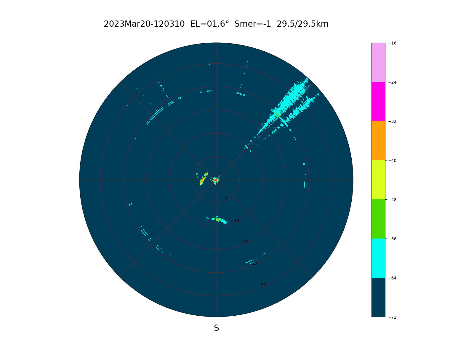
At the maximum range of 29.5km only some interference is visible around 20km in all directions, probably originating from the band-switching frequency of satellite TV receivers. High-order beat harmonics from strong reflections from rows of houses are also visible:
Less fixed targets are visible at higher antenna elevations. The picture below is taken from the actual antenna position:
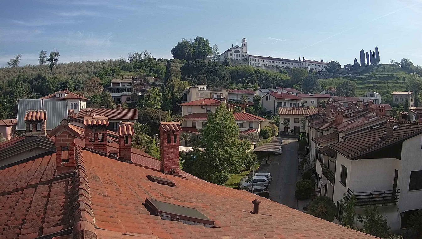
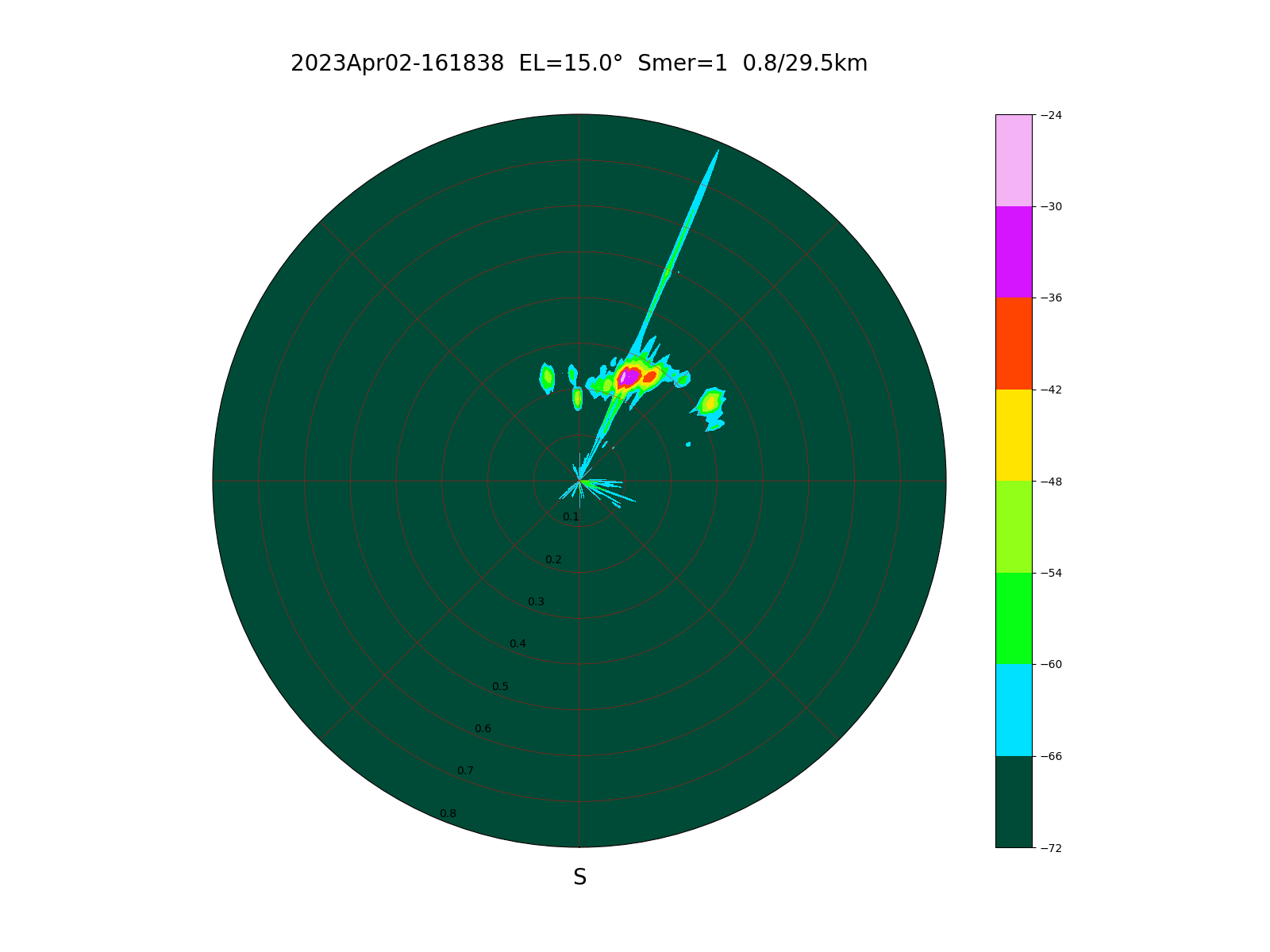
At +15 degrees elevation strong reflections from the church tower and adjacent monastery are visible within a radius of 800m. The reflections from the church tower are so strong that the FMCW radar electronics is driven into saturation, making the second harmonic of the FMCW beat signal also visible:
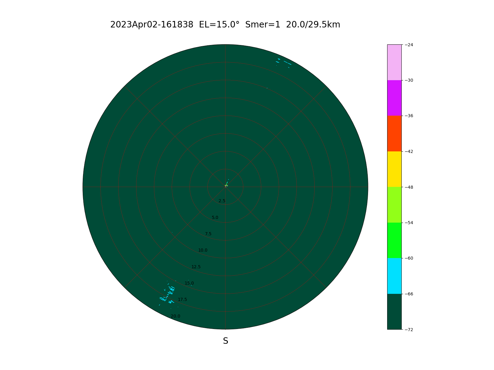
At +15 degrees elevation not much more is visible within a range of 20km in the absence of precipitations. A rather interesting detail is the Arago-diffraction backlobe from perfectly circular antennas occurring at an opposite azimuth and an opposite elevation of -15 degrees. At -15 degrees elevation there is a strong reflection from the row of houses resulting in high-order harmonics of the FMCW beat signal:
From the above discussion it is obvious that very low elevations around 0 degrees are only useful for observing ground targets. An accurate elevation setting and higher elevations are required to observe weather effects like precipitations.
(RADAR) (RF-HEAD) (ANTENNAS) (PROCESSING) (WEATHER) (HOME)